A Matrix Based Model Of Soft Body Physics
Ever since I was little, I’ve been enamored with physics simulations. There’s something so innately satisfying about having a world at your fingertips to interact with as you please. That interest has rekindled in me over the past few days as I’ve been thinking about coding up a little physics toy to mess around with now that I’m a much better programmer than I was when I was 10.
This lead me down the road of considering different ways to model physical bodies. Using bounding boxes may be a tried and true method, but who am I for taking the well worn path?
My train of thought has lead me to the idea of considering each each soft body object as a set \(\left \{ V, C \right \}\) where \(V\) is an \(n\)-dimensional vector of nodes.
A node is a \(4\)-tuple \(\left( \pi, \delta, \alpha, \rho \right)\) where \(\pi \in \mathbb{R \times R}\) is the position of the node, \(\delta \in \mathbb{R \times R}\) is the velocity of the node, and \(\alpha \in \mathbb{R \times R}\) is the acceleration of the node. The mass of the node is \(\rho \in \mathbb{R}\).
More importantly, though, is the \(n\times n\)-dimensional \(C\) matrix representing connections between nodes.
Each row and column of \(C\) corresponds to a node entry in \(V\). Entry \(C_{ij}\) corresponds to the distance that the \(i\)th node wants to be from the \(j\)th node. This is represented by:
\[C = \begin{bmatrix} C_{00} & C_{01} & C_{02} & \dots & C_{0n} \\ C_{10} & C_{11} & C_{12} & \dots & C_{1n} \\ C_{20} & C_{21} & C_{22} & \dots & C_{2n} \\ \vdots & \vdots & \vdots & \ddots & \vdots \\ C_{n0} & C_{n1} & C_{n2} & \dots & C_{nn} \end{bmatrix}\]Some immediate comments:
- The main diagonal of \(C\) is uniformly \(0\).
- \(C_{ij} = C_{ji}\)
Stepping forward the \(\pi\) and \(\delta\) elements of the nodes of \(V\) by time \(t\) is likely simple Euler integration.
To step forward \(\alpha\) in every node of \(V\), we update all of \(V\)’s \(\alpha\) values using a new vector \(V_{\alpha_t}'\) comprised of the new \(\alpha\) values after time \(t\).
Producing \(V_{\alpha_t}'\) #
Step 1: Bringing \(C\) to the spatial vector space #
We want to transform \(C\) into a matrix that deals with physical coordinates, instead of abstract values describing distances between nodes. The \(C\) that we want I will denote \(C_{\text{offset}}\).
\(C_{\text{offset}_{ij}}\) represents the offset of the position of the \(i\)th node imposed by the constraint \(C_{ij}\). This matrix \(C_\text{offset}\) can be computed as:
\[C_\text{offset} = \begin{bmatrix} (0,0) & \pidiff{0}{1} & \pidiff{0}{2} & \dots & \pidiff{0}{n} \\ \pidiff{1}{0} & (0,0) & \pidiff{1}{2} & \dots & \pidiff{1}{n} \\ \pidiff{2}{0} & \pidiff{2}{1} & (0,0) & \dots & \pidiff{2}{n} \\ \vdots & \vdots & \vdots & \ddots & \vdots \\ \pidiff{n}{0} & \pidiff{n}{1} & \pidiff{n}{2} & \dots & (0,0) \end{bmatrix}\]In general, \(C_{\text{offset}_{ij}} = \pidiff{i}{j}\). This is derived in the footnotes.
Step 2: Sum of force #
At a high level, the force applied on each node is going to be in the direction of the sum of each of the offsets, multiplied by some factor. For some node 0 \(\left( \pi, \delta, \alpha, \rho \right)\) and some constraint matrix \(C\):
\[\sum \text{Force} = C_{\text{offset}_{00}} + C_{\text{offset}_{01}} + \dots + C_{\text{offset}_{0n}}\] \[\sum \alpha = \frac{1}{\rho}\left(C_{\text{offset}_{00}} + C_{\text{offset}_{01}} + \dots + C_{\text{offset}_{0n}}\right)\]So, finding a vector of all the accelerations applied to all the nodes in order is as simple as:
\[V_\alpha' = C_\text{offset}V_\rho^{-1}\]where, to be clear, \(V_\rho^{-1}\) is the component-wise reciprocal of \(V_\rho\).
Step 3: Wrapping it all up #
Given some time interval \(t\), it is simple to make \(V_\alpha'\) depend on time by defining
\[V_{\alpha_t}' = V_\alpha't\]Applying \(V_{\alpha_t}'\) #
We will update \(V\) by linearly interpolating the values of \(V_\alpha\) with the values of \(V_{\alpha_t}'\) using some damping value \(d \in \left[0,1\right]\). Any choice of sigmoid function could have been used in place here, but I like linear interpolation because it allows for this sort damping very naturally.
So, after all this has been said and done, given a \(V = \begin{bmatrix} \left( \pi_0, \delta_0, \alpha_0, \rho_0 \right) \\ \left( \pi_1, \delta_1, \alpha_1, \rho_1 \right) \\ \vdots \\ \left( \pi_n, \delta_n, \alpha_n, \rho_n \right) \end{bmatrix}\), we have:
\[V_t' = \begin{bmatrix} \left( \pi_0, \delta_0, \lerp{\alpha_0}{V_{\alpha_{t_0}}'}{d} , \rho_0 \right) \\ \left( \pi_1, \delta_1, \lerp{\alpha_1}{V_{\alpha_{t_1}}'}{d}, \rho_1 \right) \\ \vdots \\ \left( \pi_n, \delta_n, \lerp{\alpha_n}{V_{\alpha_{t_n}}'}{d}, \rho_n \right) \end{bmatrix}\]Aren’t you usually too busy writing code to play with math? #
Yeah, but hopefully I find the time to implement this soon. Check back for links once finals end.
Sorry to end this blog post so abruptly, but I really have nothing else to say yet until I have code to show for it. Just wanted to share this idea that I had with you all.
I will type up how I derived \(\pidiff{i}{j}\) as soon as I figure out how to embed diagrams in MathJaX. Until then, consider this: it is essentially a scalar projection on the difference between two position vectors. Here’s the diagram I drew out to get some graphical intution, though it is not 100% consistent with the final results.
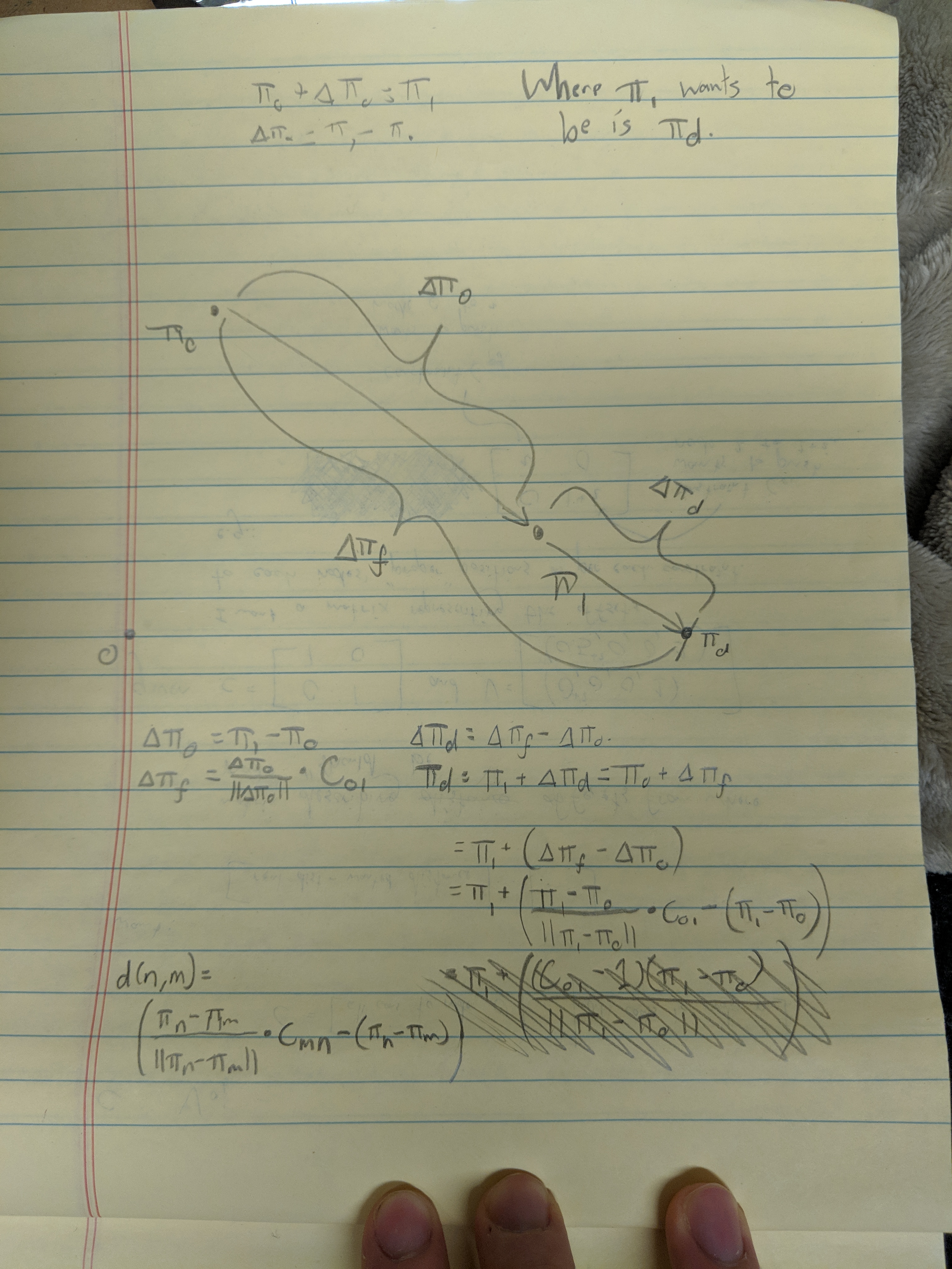